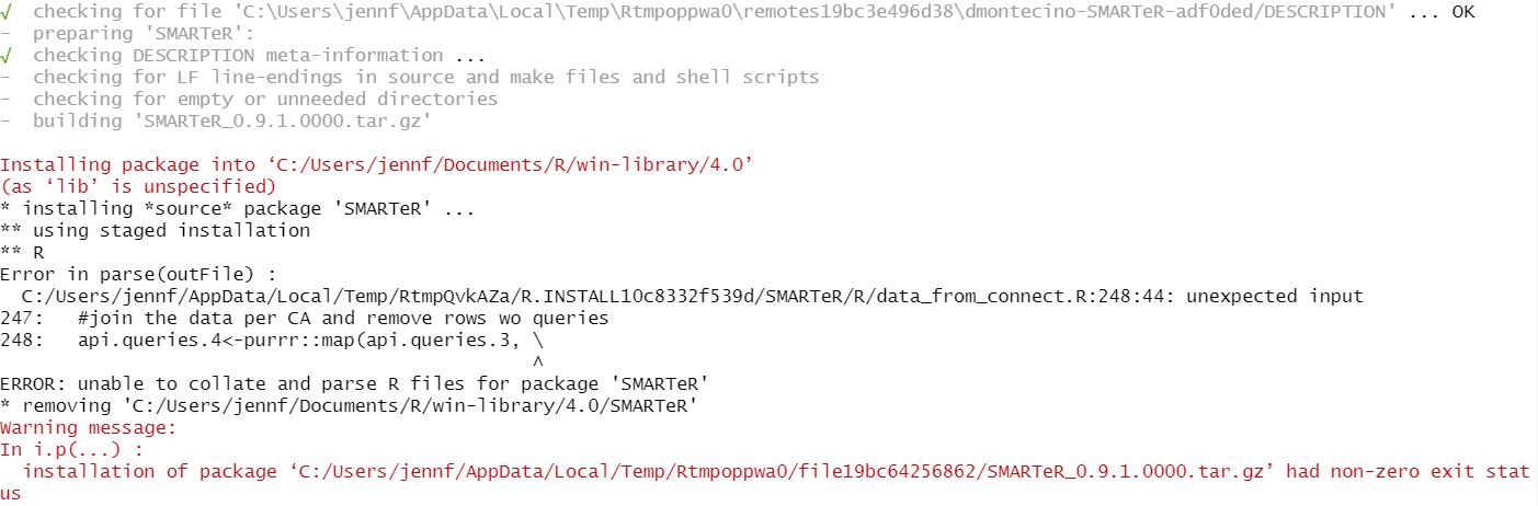
thanks for sharing this looks really helpful. However, I’m not able to install the package - I get an error message “unable to collate and parse R files for package ‘SMARTeR’”
any ideas how to get past this?
thanks for sharing this looks really helpful. However, I’m not able to install the package - I get an error message “unable to collate and parse R files for package ‘SMARTeR’”
any ideas how to get past this?
Thanks for letting me know! I will check it put right now.
When I hit install I get a message about package updates - then whether or not I update any of them I get this afterwards
I think you need to update R. If the error is amazingly well identified, then “function(x)” is equivalent to “\(x)” since R 4.1
Okay I’ll give that a try - thanks! Yes looks like I have R version 4.0.3
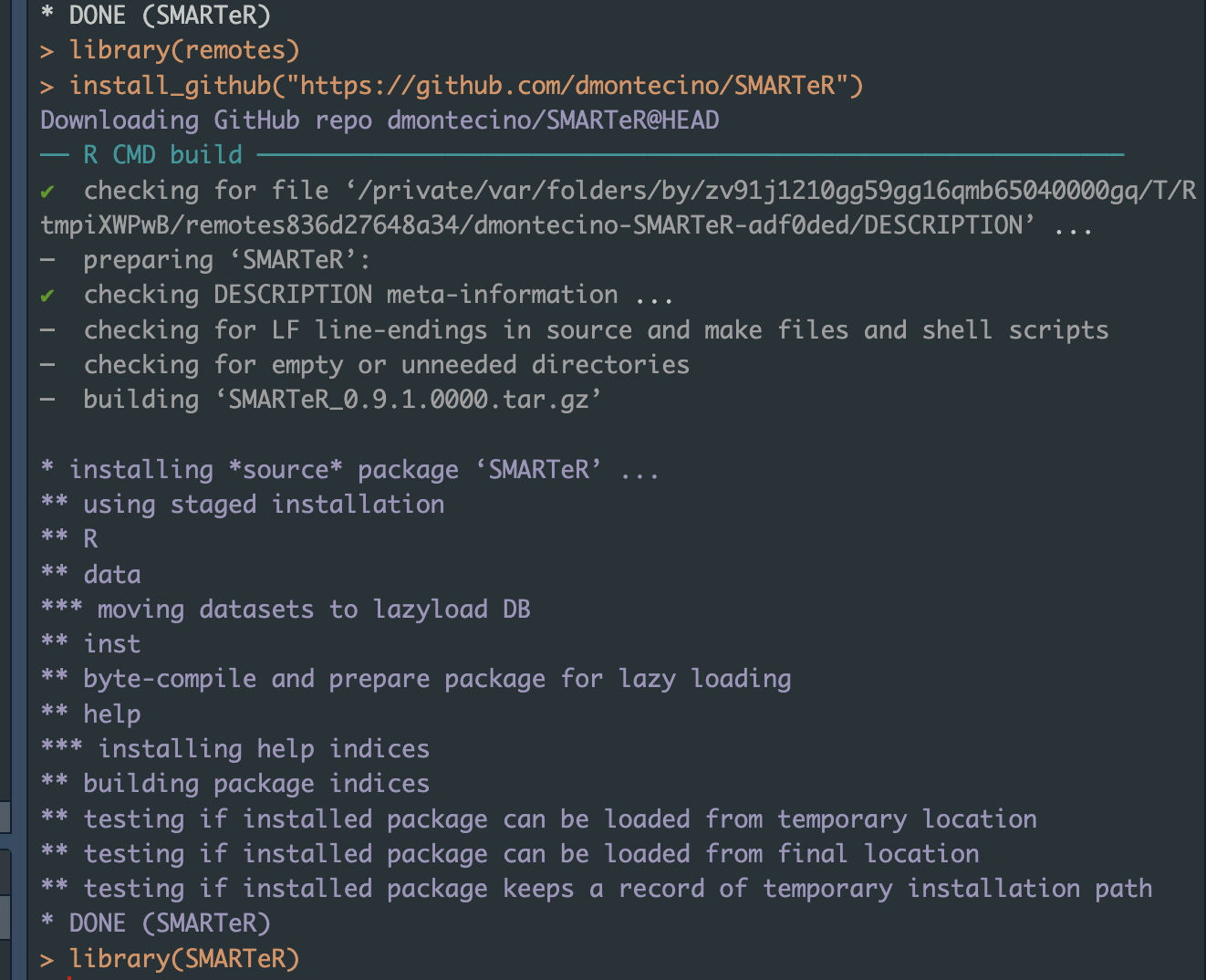
thank you that worked perfectly and I was able to query and bring in a csv file of the observations as well. this is really great!
Yes please. Id like to have those materials.
Hi Mr Russell
i did used your script with my data and ran the script but i got this errors
ERROR: Error in match.names(clabs, names(xi)) :
ERROR: The names do not match the previous names
ERROR: Calls: rbind → rbind → match.names
ERROR: Execution stop
this is the script
######################################
######################################
suppressMessages(require(ggplot2))
suppressMessages(require(tidyverse))
suppressMessages(require(ggpmisc))
suppressMessages(require(gtools))
args = commandArgs(trailingOnly=TRUE)
myquery1 = args[1]
myquery2 = args[2]
myquery3 = args[3]
myquery4 = args[4]
#The SMART query is in CSV format, so parse the
#query into a data frame
dat_traps ← read.csv(myquery1)
dat_traps$ID ← “Traps” # add ID column
names(dat_traps)[3] ← “n” # change quantity column to n
dat_camps ← read.csv(myquery2)
dat_camps$ID ← “Camps” # add ID column
names(dat_camps)[3] ← “n” # change quantity column to n
dat_offenders ← read.csv(myquery3)
dat_offenders$ID ← “Offenders” # add ID column
names(dat_camps)[3] ← “n” # change quantity column to n
effort ← read.csv(myquery4)
names(effort) ← c(“Waypoint.Date”, “effort_km”) # set new column names
dat ← rbind(dat_traps, dat_camps, dat_offenders)
dat ← dat%>%
group_by(Waypoint.Date, ID)%>%
summarise(n= sum(n, na.rm = TRUE))
dat ← left_join(dat, effort, by=“Waypoint.Date”)
remove_outliers ← function(x, na.rm = TRUE, …) {
qnt ← quantile(x, probs=c(.25, .75), na.rm = na.rm, …)
H ← 1.5 * IQR(x, na.rm = na.rm)
y ← x
y[x < (qnt[1] - H)] ← NA
y[x > (qnt[2] + H)] ← NA
y
}
dat$density ← dat$n/dat$effort_km
dat2 ← dat %>%
group_by(ID) %>%
mutate(density = remove_outliers(density))
p1 ← ggplot(dat2, aes (x=Waypoint.Date, y=density))+
geom_point(color=“black”, alpha=0.3, size=3)+
geom_smooth(method=“loess”, color=“grey50”,fill=“grey50”, size=1)+
scale_y_log10()+
theme_bw(base_size = 15)+
labs(x=“Date”,y=“log10 Density (quantity per km)”)+
stat_poly_eq(aes(label = paste(…eq.label…)),
formula = “y~x”, parse = TRUE, rr.digits = 2,
size=3,
label.x.npc = 0.9, label.y.npc = 0.99)+
stat_poly_eq(aes(label = paste(…adj.rr.label…)),
formula = “y~x”, parse = TRUE, rr.digits = 2,
size=3,
label.x.npc = 0.9, label.y.npc = 0.9)+
stat_poly_eq(aes(label = paste(…p.value.label…)),
formula = “y~x”, parse = TRUE, rr.digits = 2,
size=3,
label.x.npc = 0.9, label.y.npc = 0.78)+
geom_smooth(method=“lm”, color=“#CD001A”, se=F,
size=1.3, linetype=“dashed”)+
theme(panel.border = element_rect(size=1, fill=“transparent”),
strip.background = element_rect(fill=“grey80”),
strip.text = element_text(face=2),
axis.text.x = element_text(size=8))+
facet_wrap(~ID, scales = “free_y”)
x11()
p1
sys.sleep(10)
setwd(“Enter/File/folder/Path/Here”)
ggsave(“plot1.png”)
this is the data